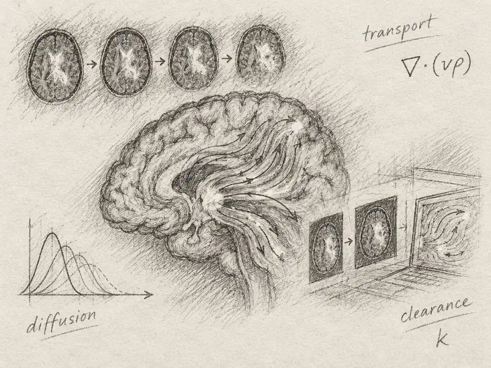
A brain MRI can show where a tracer is bright at one moment, then where it appears later. But those snapshots do not reveal the route it took between them. Did it drift with fluid, spread through tissue, or leave one region as more entered another? To answer, researchers are asking mathematics to reconstruct the hidden motion behind the pictures.
The challenge is an inverse problem. In a forward problem, scientists start with a proposed flow, simulate how a tracer would move and spread, then predict what an image should show. The inverse problem runs backward: given the images, infer the flow and other processes that could have produced them. It is a bit like watching two frames from a film and trying to recover the movement that connects them—except the object can blur, diffuse, and change in amount along the way.
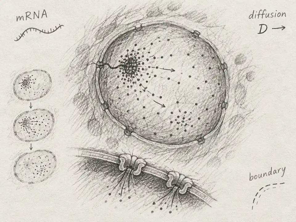
One mathematical idea at the center of this work is optimal transport: a way to describe how a distribution of material can move from one arrangement to another. In brain imaging, though, a tracer does not simply travel from point A to point B. It can spread by diffusion, and it can enter or exit the region being studied. A useful reconstruction must account for those possibilities and respect physical constraints, rather than drawing the neatest-looking path between two images.
A May 2026 arXiv study by A. Derya Bakiler and colleagues brings tools from computational mechanics into this problem. The team analyzed contrast-enhanced MRI data tracking a tracer in a mouse brain, then used an inverse model to estimate spatially varying fluid velocity, diffusion, and clearance. Their method represents the brain’s irregular geometry with smooth spline-based building blocks. That smoothing matters: image noise can make tiny voxel-to-voxel changes look like sharp turns or implausible bursts of flow.
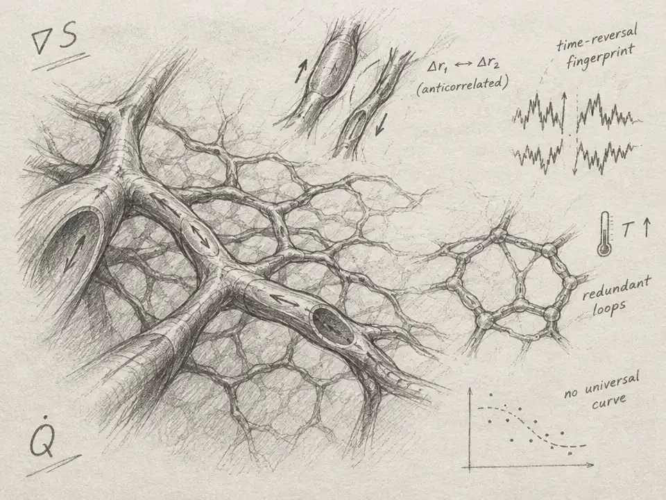
The researchers also focused on a basic accounting rule: tracer should not mysteriously appear or vanish inside the modeled tissue. Their framework builds in mass conservation and seeks velocity fields that are close to divergence-free, a mathematical way of expressing that fluid is not spuriously piling up or spreading out. In tests, forward simulations using the inferred fields tracked the observed tracer patterns. The model’s predictions also depended on which imaging times were used for calibration; a longer calibration window changed the inferred balance between diffusion and directed transport. In their analysis, diffusion remained important, even when directed flow became more prominent in some regions.
A September 2026 arXiv paper by Mehmet Emin Acar and colleagues takes a different route to the same hidden-mechanism problem. Instead of estimating a fresh transport map for each pair of images, their method, called PI-NOMT, learns continuous fields for tracer density, velocity, and local sources or sinks. It then simulates the tracer’s evolution in small steps, checking whether those fields can repeatedly generate the observed sequence. The researchers describe this as treating transport itself as a hidden state to infer, not merely using a model to fill in missing images.
Here the crossover is especially striking: ideas from optimal transport meet the machinery of scientific machine learning and the equations of fluid physics. The method first creates a continuous representation of the measured tracer images, including times between scans. Then it proposes velocity and source fields and tests them by running a differentiable simulation—one whose errors can guide the model toward a better explanation. Physical rules act like guardrails: a field that matches the images but violates the modeled transport equations is penalized.
The team first tested the approach on a synthetic moving cloud, where the true motion was known. The model could then be checked against the answer rather than judged only by how convincing its images looked. Next, the researchers applied it to tracer MRI sequences from nine control rats. Their short-interval reconstruction error averaged below 1% across the animals. But accuracy weakened over a long, uninterrupted simulation: the average normalized error across that rollout was about 11.8%. Small mismatches can compound when each simulated step becomes the starting point for the next.
That distinction is important. A model can closely match nearby snapshots without proving that it has found the one true route the tracer took. The Acar team explicitly notes that concentration images alone do not uniquely determine the underlying velocity and source fields. Different combinations of motion, diffusion, and local gain or loss may explain similar observations. The inferred paths are therefore physically constrained explanations of the data—not direct measurements of fluid movement in a living brain.
The two studies illuminate different parts of the same mathematical task. Bakiler and colleagues emphasize conservation, smooth spatial fields, and parameter recovery in a mouse-brain model. Acar and colleagues use continuous neural fields and recursive simulation across sequences from rats. Both turn image analysis into a test of mechanisms: can a proposed hidden process reproduce what the scanner observed while remaining compatible with the chosen physical rules?
The wider scientific payoff is not a finished map of brain-wide waste clearance. The biological pathways and mechanisms remain active research questions, and both approaches need broader testing. Instead, the advance is methodological: researchers can use sparse images not just to describe where a tracer is, but to ask what kinds of transport could have placed it there. Mathematics does not make the unseen flow directly visible. It makes competing explanations precise enough to test—and exposes where the evidence still runs out.